OAK enrichment command

This notebook is intended as a supplement to the main OAK CLI docs.

This notebook provides examples for the enrichment command which produces a summary of ontology classes that are enriched in the associations for an input set of entities.

See also the end of the Command Line Tutorial

Help Option

You can get help on any OAK command using --help

!runoak enrichment --help

Usage: runoak enrichment [OPTIONS] [TERMS]...

  Run class enrichment analysis.

  Given a sample file of identifiers (e.g. gene IDs), plus a set of
  associations (e.g. gene to term associations, return the terms that are
  over-represented in the sample set.

  Example:

      runoak -i sqlite:obo:uberon -g gene2anat.txt -G g2t enrichment -U my-
      genes.txt -O csv

  This runs an enrichment using Uberon on my-genes.txt, using the
  gene2anat.txt file as the association file (assuming simple gene-to-term
  format). The output is in CSV format.

  It is recommended you always provide a background set, including all the
  entity identifiers considered in the experiment.

  You can specify --filter-redundant to filter out redundant terms. This will
  block reporting of any terms that are either subsumed by or subsume a lower
  p-value term that is already reported.

  For a full example, see:

     https://github.com/INCATools/ontology-access-
     kit/blob/main/notebooks/Commands/Enrichment.ipynb

  Note that it is possible to run "pseudo-enrichments" on term lists only by
  passing no associations and using --ontology-only. This creates a fake
  association set that is simply reflexive relations between each term and
  itself. This can be useful for summarizing term lists, but note that
  P-values may not be meaningful.

Options:
  -o, --output FILENAME           Output file, e.g. obo file
  -p, --predicates TEXT           A comma-separated list of predicates. This
                                  may be a shorthand (i, p) or CURIE
  --autolabel / --no-autolabel    If set, results will automatically have
                                  labels assigned  [default: autolabel]
  -O, --output-type TEXT          Desired output type
  -o, --output FILENAME           Output file, e.g. obo file
  --ontology-only / --no-ontology-only
                                  If true, perform a pseudo-enrichment
                                  analysis treating each term as an
                                  association to itself.  [default: no-
                                  ontology-only]
  --cutoff FLOAT                  The cutoff for the p-value; any p-values
                                  greater than this are not reported.
                                  [default: 0.05]
  -U, --sample-file FILENAME      file containing input list of entity IDs
                                  (e.g. gene IDs)  [required]
  -B, --background-file FILENAME  file containing background list of entity
                                  IDs (e.g. gene IDs)
  --association-predicates TEXT   A comma-separated list of predicates for the
                                  association relation
  --filter-redundant / --no-filter-redundant
                                  If true, filter out redundant terms
  --help                          Show this message and exit.

Download example file and setup

We will use the HPO Association file

!curl -L -s http://purl.obolibrary.org/obo/hp/hpoa/genes_to_phenotype.txt > input/hpoa_g2p.tsv

next we will set up an hpo alias

alias hp runoak -i sqlite:obo:hp

Test this out by querying for associations for a particular gene.

We need to pass in the association file we downloaded, as well as specify the file type (with -G):

hp -G hpoa_g2p -g input/hpoa_g2p.tsv associations -Q subject NCBIGene:8192 -O csv | head

subject subject_label   predicate       object  object_label    property_values predicate_label negated publications    primary_knowledge_source        aggregator_knowledge_source     subject_closure subject_closure_label   object_closure  object_closure_label
NCBIGene:8192   None    None    HP:0001250      None            None    None            None    None
NCBIGene:8192   None    None    HP:0000013      None            None    None            None    None
NCBIGene:8192   None    None    HP:0000007      None            None    None            None    None
NCBIGene:8192   None    None    HP:0010464      None            None    None            None    None
NCBIGene:8192   None    None    HP:0008232      None            None    None            None    None
NCBIGene:8192   None    None    HP:0011969      None            None    None            None    None
NCBIGene:8192   None    None    HP:0004322      None            None    None            None    None
NCBIGene:8192   None    None    HP:0000786      None            None    None            None    None
NCBIGene:8192   None    None    HP:0000815      None            None    None            None    None

Enrichment

We will perform enrichment using a set of genes known to be associated with Ehler-Danlos Syndrome (EDS).

The gene list is here:

• input/eds-genes-ncbigene.tsv

Let’s take a look at them:

!cat input/eds-genes-ncbigene.tsv

id      label
NCBIGene:7148   TNXB
NCBIGene:715    C1R
NCBIGene:716    C1S
NCBIGene:126792 B3GALT6
NCBIGene:55033  FKBP14
NCBIGene:91252  SLC39A13
NCBIGene:29940  DSE
NCBIGene:1303   COL12A1
NCBIGene:9509   ADAMTS2
NCBIGene:1278   COL1A2
NCBIGene:1281   COL3A1
NCBIGene:1289   COL5A1
NCBIGene:1290   COL5A2
NCBIGene:84627  ZNF469
NCBIGene:113189 CHST14
NCBIGene:165    AEBP1
NCBIGene:5351   PLOD1
NCBIGene:11285  B4GALT7
NCBIGene:11107  PRDM5

Running the enrichment command

Next we will run the command itself. Note we use two sets of parameters

• global OAK parameters:

  • the format of the associations (-G), here using the HPOA gene to phenotype format

  • the path to the association file (-g), here the gp2 file we downloaded earlier

• local parameters for the enrichment command

  • the set of genes to be enriched (via -U or --sample-file)

  • the output format for the results (via -O or --output-type) - here a TSV, but could also be YAML, RDF

  • the --autolabel option that will do additional HPO queries to give the names of each term

  • the output file via -o (--output)

hp -G hpoa_g2p -g input/hpoa_g2p.tsv enrichment -U input/eds-genes-ncbigene.tsv -O csv --autolabel -o output/eds-genes-enriched.tsv

Examining the results

The best way to look at TSVs in a notebook such as this one is to use pandas to load as a dataframe. Note however that in most scenarios where you use the command line, this would not be wrapped in a notebook, and you could use your favorite TSV/CSV tool for exploring the results

import pandas as pd

df=pd.read_csv("output/eds-genes-enriched.tsv", sep="\t")
df

	class_id	p_value	class_label	rank	p_value_adjusted	false_discovery_rate	fold_enrichment	probability	sample_count	sample_total	background_count	background_total	ancestor_of_more_informative_result	descendant_of_more_informative_result
0	HP:0000974	2.121426e-37	Hyperextensible skin	1	2.895747e-34	NaN	NaN	NaN	19	19	68	5011	NaN	NaN
1	HP:0001075	1.245666e-36	Atrophic scars	2	1.700334e-33	NaN	NaN	NaN	17	19	37	5011	NaN	NaN
2	HP:0008067	9.834712e-29	Abnormally lax or hyperextensible skin	3	1.342438e-25	NaN	NaN	NaN	19	19	177	5011	True	NaN
3	HP:0100699	1.916985e-28	Scarring	4	2.616685e-25	NaN	NaN	NaN	19	19	183	5011	True	NaN
4	HP:0004334	7.330381e-28	Dermal atrophy	5	1.000597e-24	NaN	NaN	NaN	17	19	102	5011	True	NaN
...	...	...	...	...	...	...	...	...	...	...	...	...	...	...
159	HP:0010488	3.040076e-05	Aplasia/Hypoplasia of the palmar creases	160	4.149704e-02	NaN	NaN	NaN	3	19	17	5011	NaN	True
160	HP:0000014	3.062457e-05	Abnormality of the bladder	161	4.180254e-02	NaN	NaN	NaN	9	19	494	5011	True	NaN
161	HP:0011844	3.186952e-05	Abnormal appendicular skeleton morphology	162	4.350189e-02	NaN	NaN	NaN	16	19	1853	5011	True	NaN
162	HP:0033353	3.286903e-05	Abnormal blood vessel morphology	163	4.486623e-02	NaN	NaN	NaN	12	19	967	5011	True	True
163	HP:0025323	3.300320e-05	Abnormal arterial physiology	164	4.504937e-02	NaN	NaN	NaN	6	19	177	5011	True	True

164 rows × 14 columns

Plotting the results

OAK doesn’t have any command line plotting capabilities yet, but you can easily use external tools. Here we show how to plot the results using matplotlib.

import matplotlib.pyplot as plt
import numpy as np

data = df.copy()

# Transform p-values for better visualization
data['negative_log10_p_value'] = -np.log10(data['p_value'])

# Sort data by transformed p-value
data_sorted = data.sort_values('negative_log10_p_value', ascending=True)

# Select top 15 terms with the highest significance
top_terms = data_sorted.nlargest(15, 'negative_log10_p_value')

# Plotting the horizontal bar chart for the top 15 terms
plt.figure(figsize=(10, 10))
plt.barh(top_terms['class_label'], top_terms['negative_log10_p_value'], color='teal')
plt.xlabel('-log10(p-value)')
plt.ylabel('Enriched Terms')
plt.title('Top 15 Enriched Terms by Statistical Significance')
plt.gca().invert_yaxis()  # Invert y-axis for better readability
plt.show()

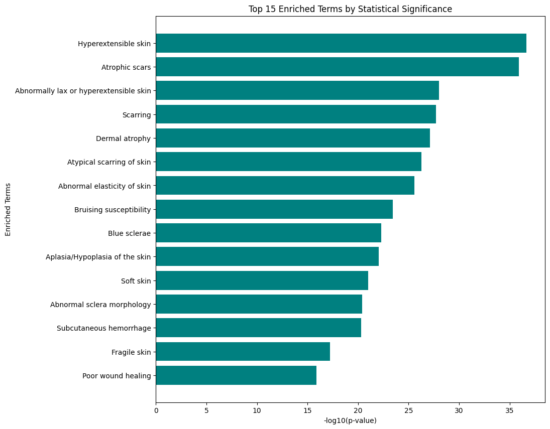
The results here should not be surprising - we already know that hyperextensible skin is a hallmark of EDS, but it’s good to see this confirmed!

We used a somewhat artificial gene set here, but in reality gene sets derived e.g. from gene expression will be more messy and signals weaker.

Visualizing results in a graph form

We can use the OAK viz command to visualize the placement of the enriched terms in the graph.

Because graph visualization can get messy, we’ll take the top 5 results (they are already sorted):

!head -5 output/eds-genes-enriched.tsv > output/eds-genes-enriched-top-5.tsv

Next run this through viz. Note that most OAK commands take as input either term lists, or term query lists, where queries can include expressions with functions like .idfile:

hp viz -p i .idfile output/eds-genes-enriched-top-5.tsv -O png -o output/eds-genes-enriched-top-5.png

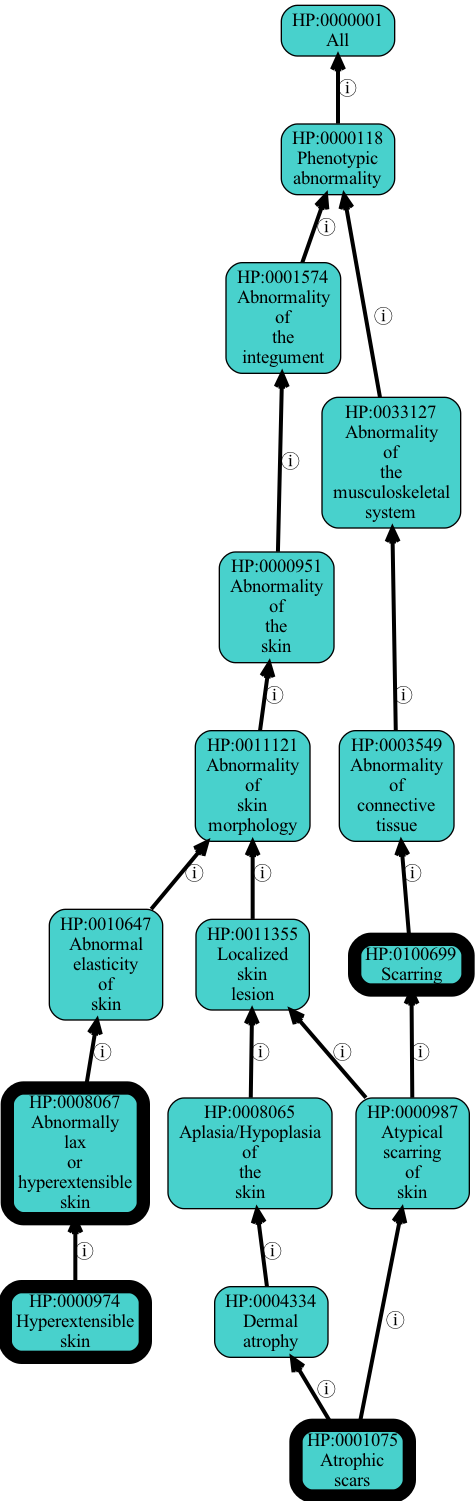
At this time there isn’t an easy way to show the p-value visually, but this may be added later.

When we visualize like this we see there is some redundancy. Scarring is implied by Atrophic scars.

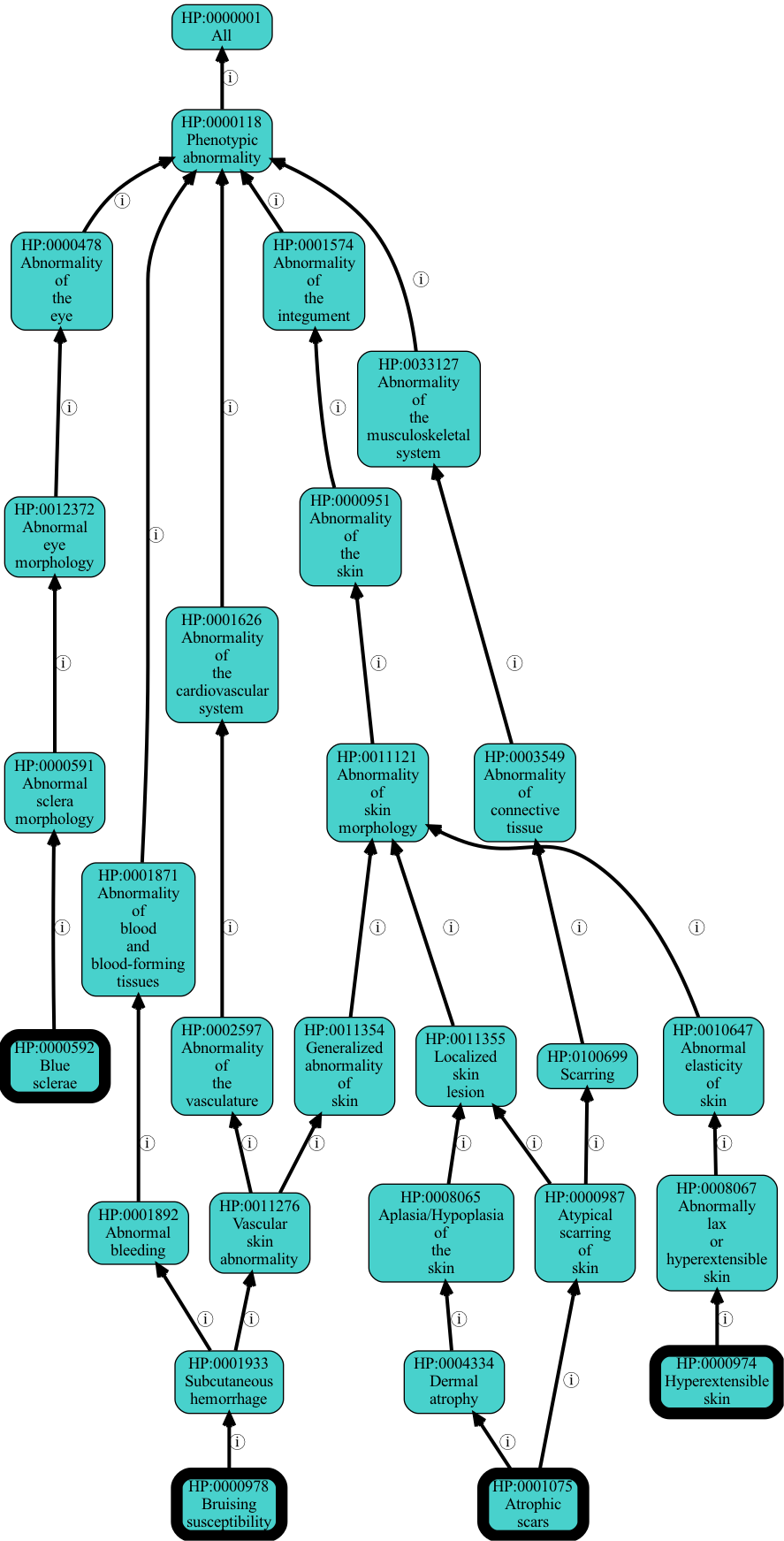
We can run enrichment with --filter-redundant on. This will remove more general terms, unless that term is more significant than all descendants.

hp -G hpoa_g2p -g input/hpoa_g2p.tsv enrichment -U input/eds-genes-ncbigene.tsv -O csv --autolabel  --filter-redundant -o output/eds-genes-enriched-filtered.tsv

!head -5 output/eds-genes-enriched-filtered.tsv > output/eds-genes-enriched-filtered-top-5.tsv

hp viz -p i .idfile output/eds-genes-enriched-filtered-top-5.tsv -O png -o output/eds-genes-enriched-filtered-top-5.png

Normalizing input gene lists

What happens if our input gene IDs use a different system than the associations?

E.g. assume our inputs are HGNC and our association file is NCBIGene

• input/eds-genes-hgnc.tsv

Let’s take a look

!cat input/eds-genes-hgnc.tsv

id      label
HGNC:11976      TNXB
HGNC:1246       C1R
HGNC:1247       C1S
HGNC:17978      B3GALT6
HGNC:18625      FKBP14
HGNC:20859      SLC39A13
HGNC:21144      DSE
HGNC:2188       COL12A1
HGNC:218        ADAMTS2
HGNC:2198       COL1A2
HGNC:2201       COL3A1
HGNC:2209       COL5A1
HGNC:2210       COL5A2
HGNC:23216      ZNF469
HGNC:24464      CHST14
HGNC:303        AEBP1
HGNC:9081       PLOD1
HGNC:930        B4GALT7
HGNC:9349       PRDM5

hp -G hpoa_g2p -g input/hpoa_g2p.tsv enrichment -U input/eds-genes-hgnc.tsv -O csv --autolabel

ValueError: No associations found for subjects

As expected, the command complains that no associations were found for any of the subjects (input genes).

So what do we do? There is a separate command normalize that can be used here to normalize an ID list. Normalize can be used with a number of different ID mapper / normalizer sources. Here we are using it with the NCATS Translator SRI node normalizer:

!runoak -i translator: normalize .idfile input/eds-genes-hgnc.tsv -M NCBIGene -o output/eds-genes-ncbigene.tsv

!cat output/eds-genes-ncbigene.tsv

id      label
NCBIGene:7148   TNXB
NCBIGene:715    C1R
NCBIGene:716    C1S
NCBIGene:126792 B3GALT6
NCBIGene:55033  FKBP14
NCBIGene:91252  SLC39A13
NCBIGene:29940  DSE
NCBIGene:1303   COL12A1
NCBIGene:9509   ADAMTS2
NCBIGene:1278   COL1A2
NCBIGene:1281   COL3A1
NCBIGene:1289   COL5A1
NCBIGene:1290   COL5A2
NCBIGene:84627  ZNF469
NCBIGene:113189 CHST14
NCBIGene:165    AEBP1
NCBIGene:5351   PLOD1
NCBIGene:11285  B4GALT7
NCBIGene:11107  PRDM5

This is identical to the gene list in the original example, and can be used in the same way